Shapley values meet NNPDF

Raphaël Bonnet-Guerrini¹,
In collaboration with: Stefano Carrazza², Dakshansh Chawda², Stefano Forte², Eva Groenendijk², Vincenzo Piuri¹, and Ramon Winterhalder²

¹Computer Science Department, University of Milan;
²TIF lab, Physics Department, University of Milan

Parton Distribution Functions (PDFs) and NNPDF

\[ f_i(x, Q_0^2) = x^{(1-a)}(\text{NN}_i(x)-\text{NN}_i(1)) \]

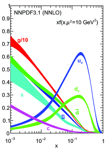
Describe the probability of finding a parton carrying a fraction \(x\) of the proton's momentum at a given energy scale \(Q^2\).
Predicts outcomes of particle collisions.
NNPDF uses NN to model PDFs without assuming a specific functional form.
Trained on data from different experiments.

PDF fitting: an inverse problem

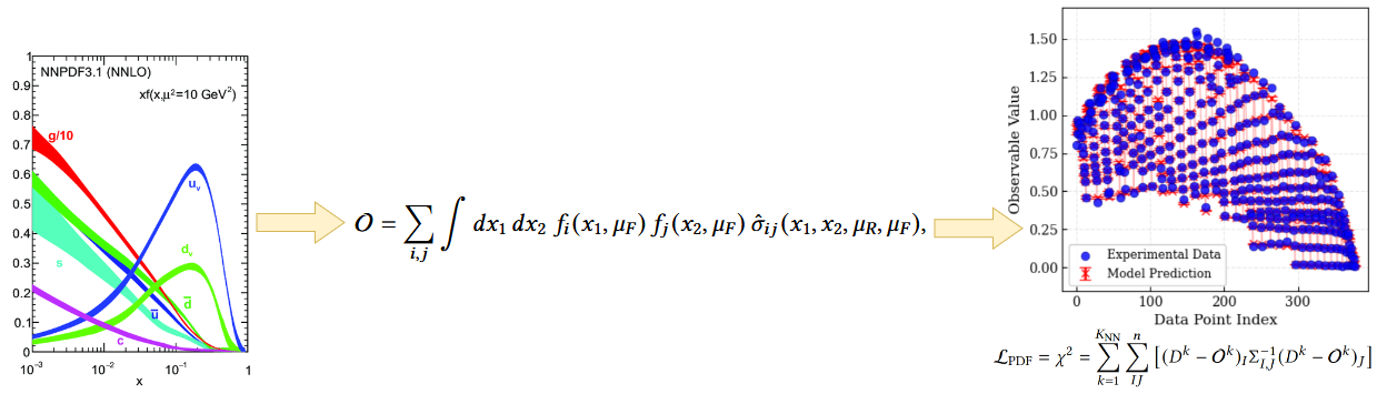
NNPDF solves an inverse problem: we have a set of experimental data and we want to find the underlying PDFs that best explain the data.

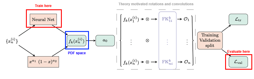
Theory (QCD, QED) allows us to compute the observable values \(\mathcal{O}_n\) from the PDF space, and the inverse is done by fitting precise experimental data.

PDF space

The PDF space is a 9-dimensional space (flavor basis or evolution basis).
Why does a given flavor look like this in a given \(x\) region? Which datasets are responsible for this behavior?

What if we perturb the PDF directly in the PDF space ?

Multidimensionality of the PDF space, Rotation and convolutions, PDF-Observable correlations, DGLAP Evolution.
Makes it difficult to perform systematic tests and obtain a clear understanding of each flavor on the fit.

NNPDF a black box model ?

Black-box systems are a recurrent interpretability issue in modern DL. We can take inspiration from the methods developed there to solve the interpretability problem of NNPDF.

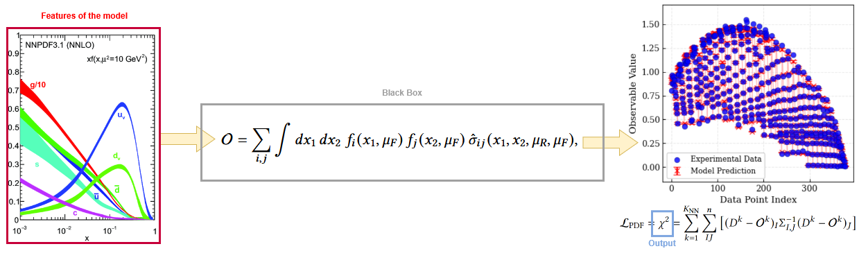
XAI answer : What's the impact of one feature on the output of the model ?

Shapley Values

Inherited from game theory: represent the value of the contribution \(\phi\) of a player \(i\) within a coalition \(S\).

\[ \phi_i = \sum_{S \subseteq N \setminus \{i\}} \frac{|S|! \, (|N| - |S| - 1)!}{|N|!} \left[ v(S \cup \{i\}) - v(S) \right] \]

where \(N\) is the set of all players, \(S\) is a subset of players not including \(i\), and \(v(S)\) is the value of the coalition \(S\).

Computational cost scales exponentially with the number of players \(2^N\).

SHAP adapts SV for DL application. Makes them computable for large numbers of players (features) given certain assumptions and approximations.

Shapley Value, the perfect closure test metric?

Applying Shapley Values to NNPDF, we treat the PDF of each flavor as an input of our black-box model.

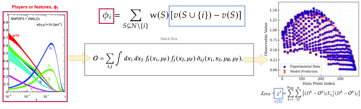
\(\phi_i\) is the Shapley Value for flavor \(i\).
\(N\) is the total number of flavors.
\(S\) is a subset of flavors not including \(i\).
\(v(S)=\chi^2\) is the value of the coalition when all flavors in coalition \(S\) are perturbed, while \(i\) and the rest of the flavors remain untouched.

The Shapley analysis in NNPDF

Loading trained PDFs from n3fit.

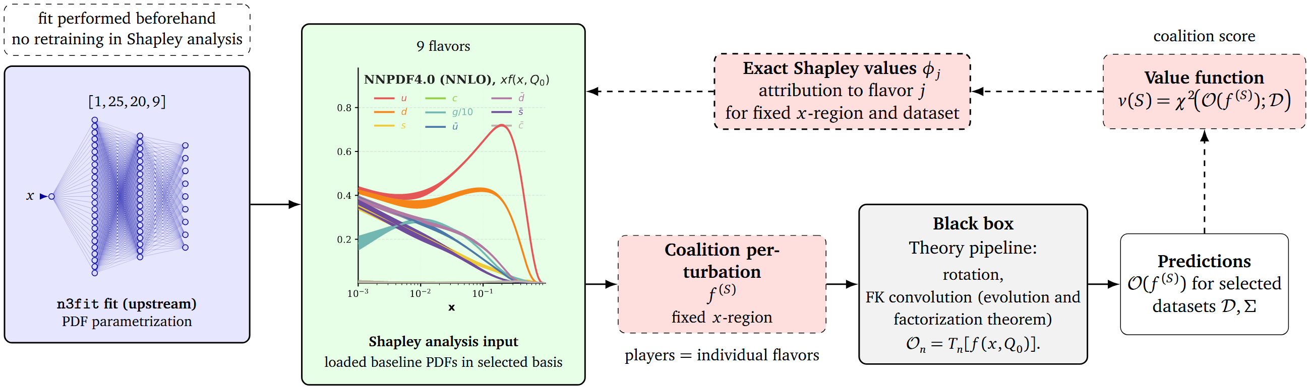
For selected datasets, we can run the following Shapley analysis:

All possible coalitions of perturbed PDFs are being created.
We compute the \(\chi^2\) for each coalition.
For each single flavor, we compare the \(\chi^2\) of the coalition, with the flavor perturbed and not perturbed.

How to perturb the PDF space ?

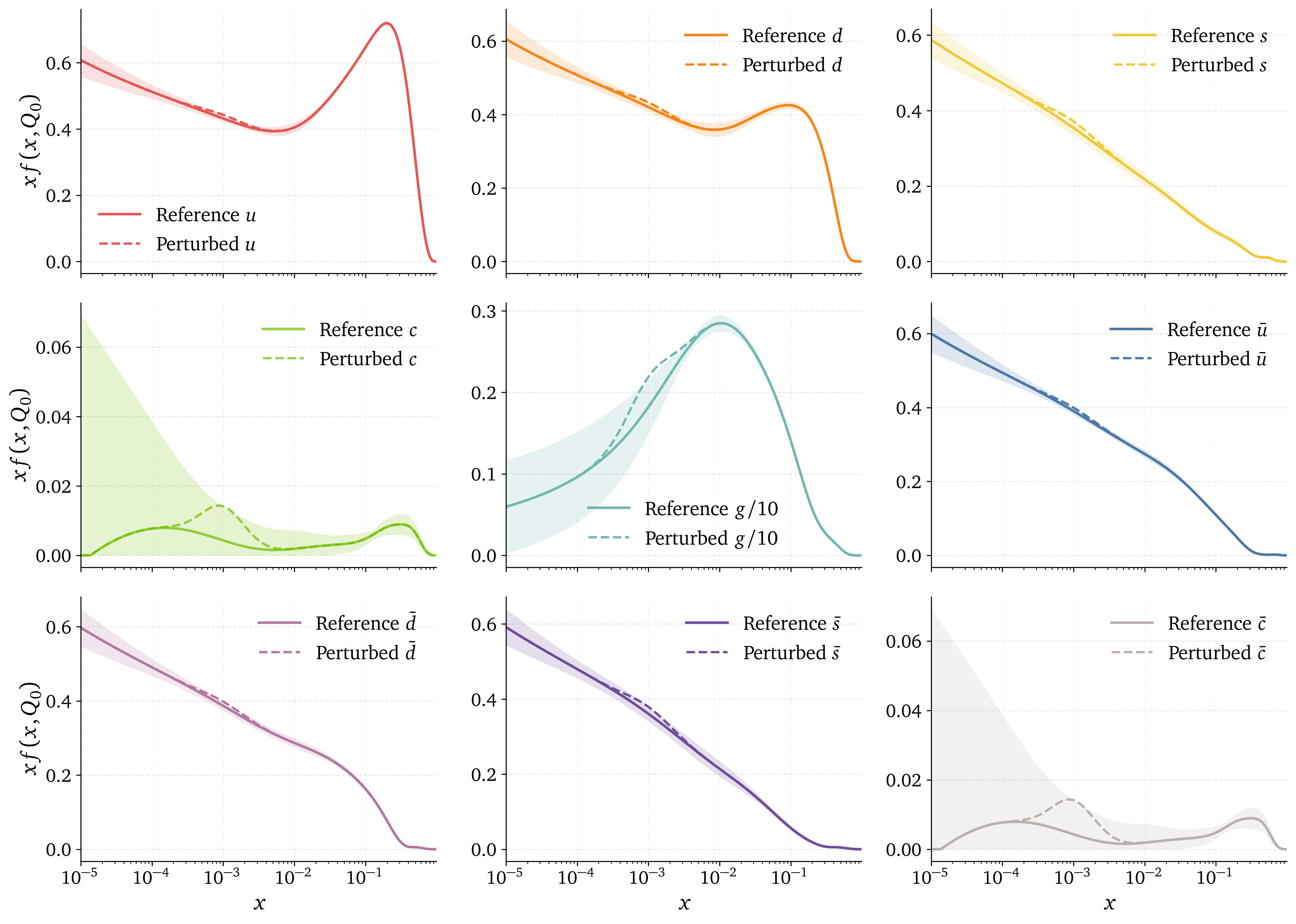
How do we perturb a PDF ? A smooth calibrated Gaussian bump:

How to perturb the PDF space ?

How do we perturb a PDF ? A smooth calibrated Gaussian bump:

\[ xf_j^{\text{pert}}(x)=xf_j(x)\pm \delta_j(x), \qquad \text{with} \quad \delta_j(x)= \sigma_{\text{rep},j}(x_{\mu}) \exp\!\left(-\frac{(x-\mu)^2}{2\sigma^2}\right). \]

How to avoid directional bias ? average the Shapley value of both directions \[ v(S)=\frac{v_+(S)+v_-(S)}{2}. \]

Coalitions and complexity

What we compute: the exact Shapley value for each PDF flavor by averaging its marginal contribution across all coalitions (all subsets of flavors).

Computational cost: exponential in the number of flavors, as we need to evaluate the fit for each coalition. In the flavor basis, \(N=9\) flavors, we have \(2^9 = 512\) coalitions.

Using exact Shapley values, we make no assumption of independence of the features.

Correlated perturbation

We can set coalitions with correlated perturbation. How to infer the correlations between the flavors:

Sum rules:

\[ \text{Momentum sum rule:} \quad\int_0^1dxx(g(x,Q)+\Sigma(x,Q))=1, \] \[ \text{Valence sum rule:} \int_0^1dxV(x,Q)=\int_0^1dxV_8(x,Q)=3, \qquad \int_0^1dxV_3(x,Q)=1, \]

Sum rules enforce physical PDF and correlate our perturbations within a coalition.

How to interpret the Shapley values?

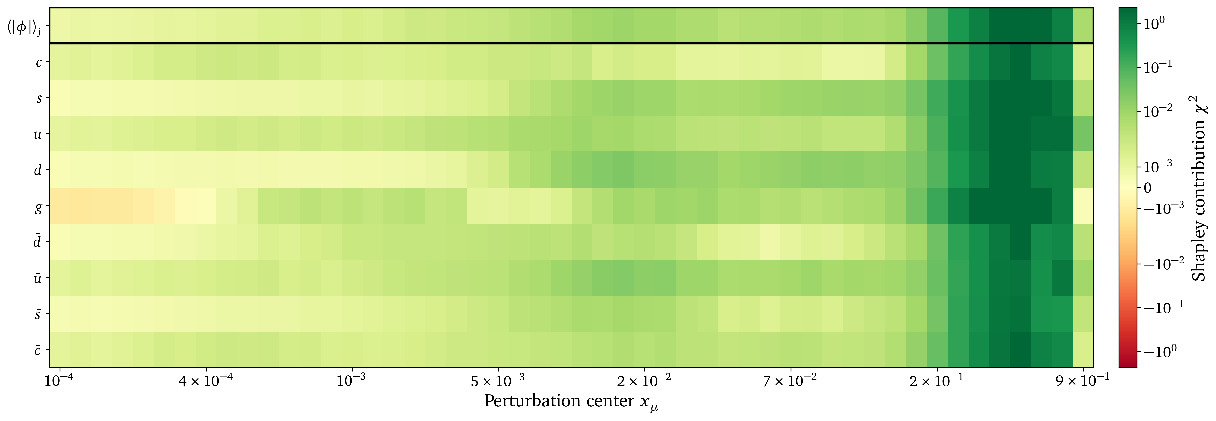
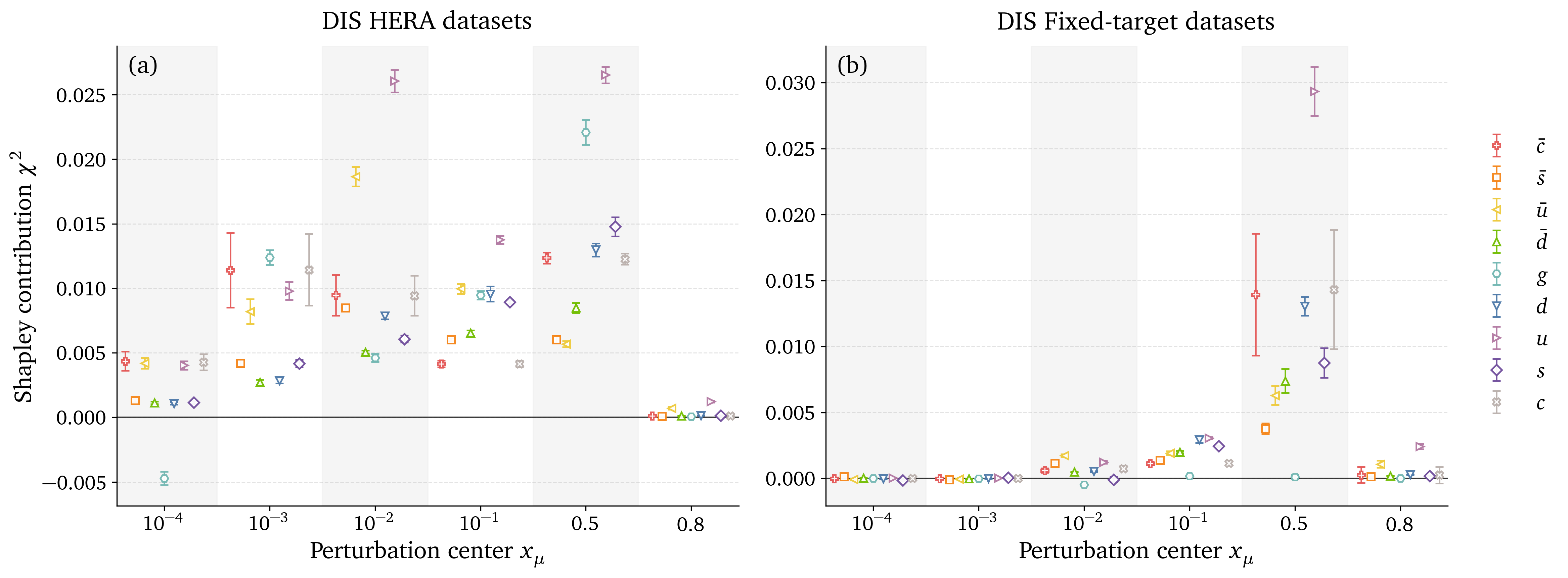
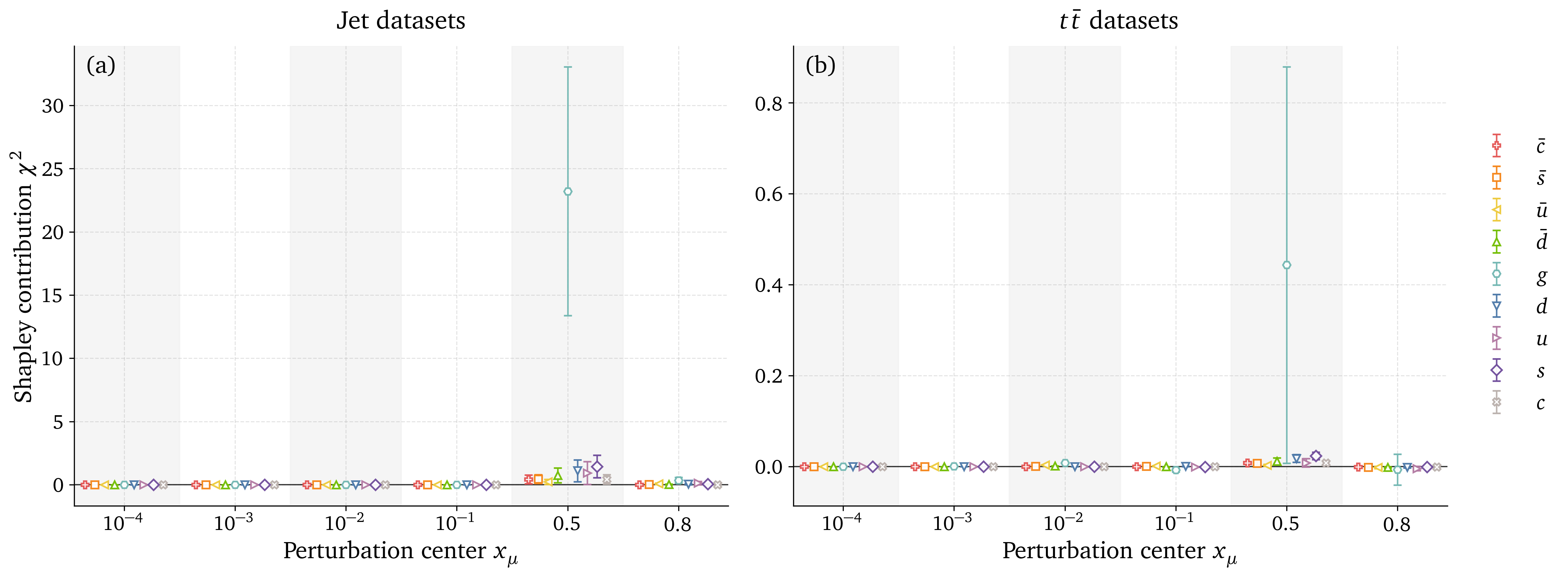
\(\phi_j< 0 \) flavor \(j\) is poorly constrained for this dataset.

\(\phi_j> 0 \) flavor \(j\) is well constrained.

\(x\) region dependency: Perturbation is local and we can expect different contributions for different \(x\) regions.

Dataset dependency: \(\chi^2\) which is computed based on experimental dataset. We expect different contributions for different datasets.

Exact Shapley Value have a completeness property: \[\sum_{j \in N} \phi_j = v(N)-v(\emptyset)\] and \(v(s)=\chi^2\) so they share the same unit.

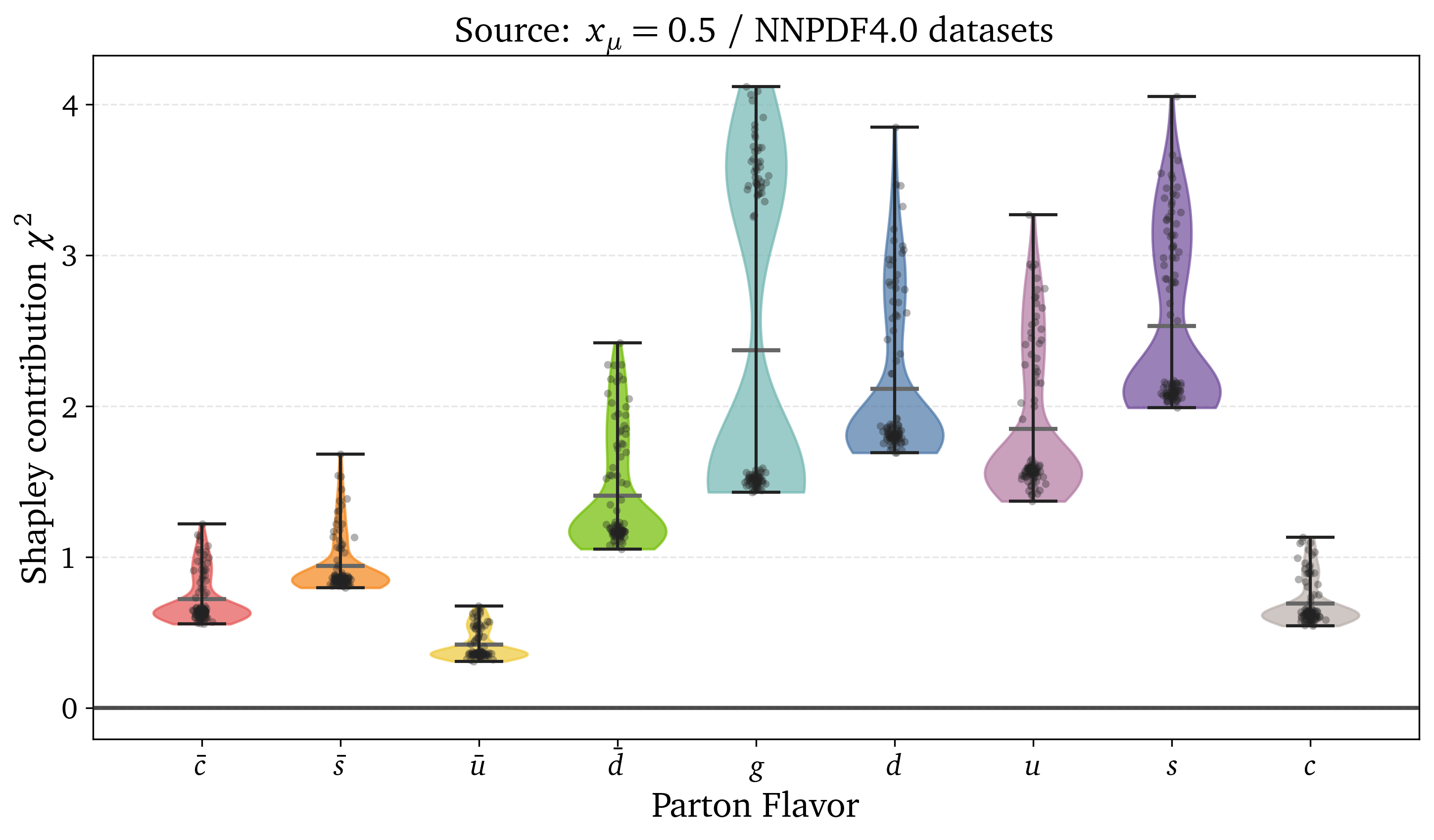
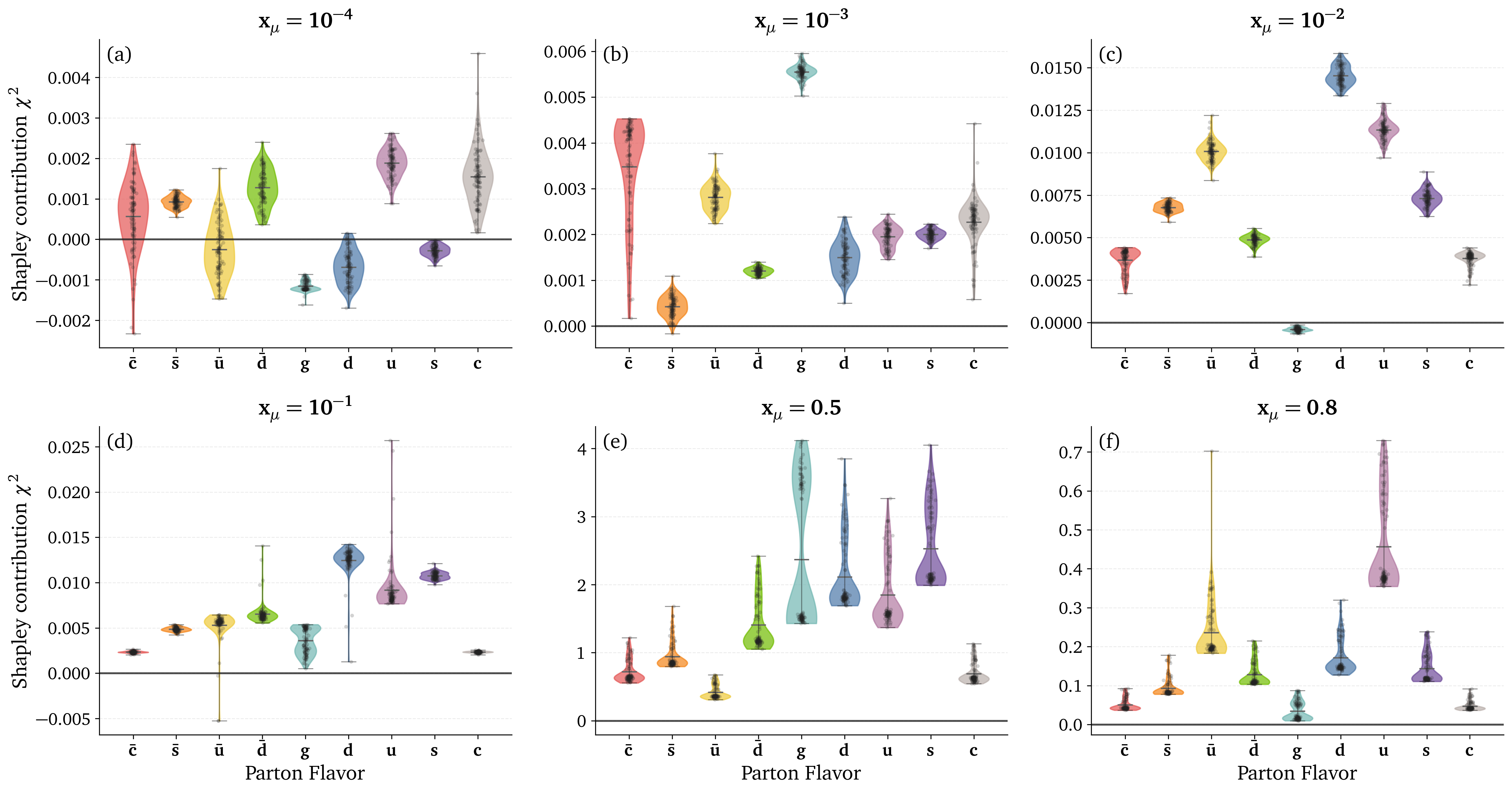
Preliminary results: Kinematic dependence

Preliminary results: DIS datasets analysis

Preliminary results: Gluon datasets analysis

Outlook

Quantitative contribution of individual flavor.
Demonstrate expected behavior on tested datasets.

Future steps

In the context of calibrated perturbation, what does it tell us about the calibration of the uncertainties of NNPDF.
Potential for quantitative K-folding repartition.

Thank you !

Contact : raphael.bonnet-guerrini@unimi.it

This work was supported by the European Union's Horizon Europe research and innovation programme under the Marie Sklodowska-Curie grant agreement No 101168829, Challenging AI with Challenges from Physics: How to solve fundamental problems in Physics by AI and vice versa (AIPHY).

Backup Slides

Shapley Values Pseudocode

# INPUT: observables, mu,sigma,amplitude, n_samples, n_flavors = n
# OUTPUT: shapley_vals[], baseline_chi2, cache

baseline_chi2 = evaluate_chi2(observables, flavor_subset=[])   # v({})

cache = {}   # map subset -> v(S)
all_subsets = power_set(0..n-1)     # exclude full-set if desired

for i in 0..n-1:
SV = 0
for S in all_subsets:
    if i in S: continue

    # v(S)
    if S not in cache:
    cache[S] = evaluate_chi2(observables, flavor_subset=list(S), mu,sigma,amplitude, n_samples)
    vS = cache[S]

    # v(S ∪ {i})
    S_with = S ∪ {i}
    if S_with not in cache:
    cache[S_with] = evaluate_chi2(observables, flavor_subset=list(S_with), mu,sigma,amplitude, n_samples)
    vSw = cache[S_with]

    Δ = vSw - vS                                   # marginal contribution
    s = |S|
    w = factorial(s) * factorial(n - s - 1) / factorial(n)
    SV += w * Δ

shapley_vals[i] = SV

# RETURN: shapley_vals, baseline_chi2, evaluated_coalitions=|cache|
# COMPLEXITY: time ~ O(n · 2^n · cost_eval), space ~ O(2^n) (memoized)

Shapley Values weight

In game theory, Shapley Values represent the contribution \(\phi_i\) of a player \(i\) within a coalition \(S\) by comparing the outcomes of scenarios where the player is present \(v(S \cup \{i\})\) versus absent \(v(S)\). \[ \phi_i = \sum_{S \subseteq N \setminus \{i\}} \text{w}(S) \left[ v(S \cup \{i\}) - v(S) \right] \label{eq:comb_SV} \] With: \[ w(S) = \frac{|S|! \, (|N| - |S| - 1)!}{|N|!} \] \(w(S)\) weights for the importance of the coalition \(S\) being tested. It is the probability that the set of players who come after \(i\) is exactly \(S\).

\(|S|!\) is the number of ways to order the predecessors of \(i\)
\((|N| - |S| - 1)!\) is the number of ways to order the players before \(i\)
\(|N|!\) is the number of ways to order all players

Shapley Values weight

This result is derived in the following way: Given \( |N| = n \), for a fixed player \(i\), let \( S \subseteq N \setminus \{i\} \) with \( |S| = s \). The probability that players before \(i\) are exactly \(S\) can be decomposed into two conditions: First, \(i\) can be in any position in \(N\), so: \[ p(\text{pos}_i = s+1) = \frac{1}{n} \] Second, given that \( i \) is in position \( s+1 \), the \( s \) players before \( i \) form a uniformly random subset of the remaining \( n-1 \) players of size \(\binom{n-1}{s}\): \[ p(\text{predecessors} = S \mid \text{pos}_i = s+1) = \frac{1}{\binom{n-1}{s}} \] To fulfill these conditions, we multiply those probabilities: \[ \frac{1}{n}\cdot \frac{1}{\binom{n-1}{s}} = \frac{1}{n}\cdot \frac{s!(n-1-s)!}{(n-1)!} = w(S) \]