Interpretable Deep Learning for Fundamental Physics
From Supernovae detection to Neutrinos passing by Parton Distribution Functions.


Research Focus: interpretability in Deep Learning
Deep Learning models are black boxes
Extremely dense set of methods.


How to do interpretability in Fundamental Physics?
Large set of methods for interpretability and explainability, but mostly non-trivial to transfer.
Reasons?
Type of data, type of problem, type of scientific downstream application, (???)
Targets?
- Reliable and calibrated uncertainties.
- Global behavior analysis and explanations.
- Identification of breaking points in models.
- ???
Interpretable Deep Learning for Real/Bogus classification with Uncertainty Quantification
Raphaël Bonnet-Guerrini1, Dominique Fouchez2, Vincenzo Piuri1, Benjamin Racine2, and Bruno Sanchez21Computer Science Department, University of Milan; 2Centre de Physique des Particules de Marseille

Cosmology: a data driven era
- Calibrate the image
- Find all differences (~10k/image)
-
For each difference
- Perform photometry
- Crossmatch with known catalogs
- Find nearest Solar System objects
- Compute various features
- Find past LSST detections at this location
- Package into an alert
Difference Image analysis
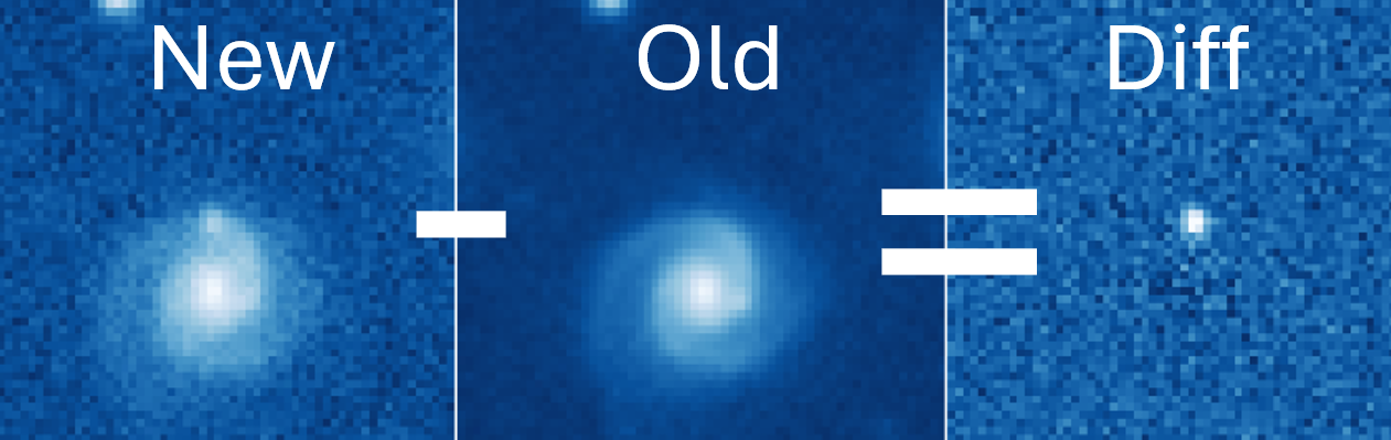
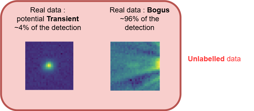
Weakly supervised learning problem
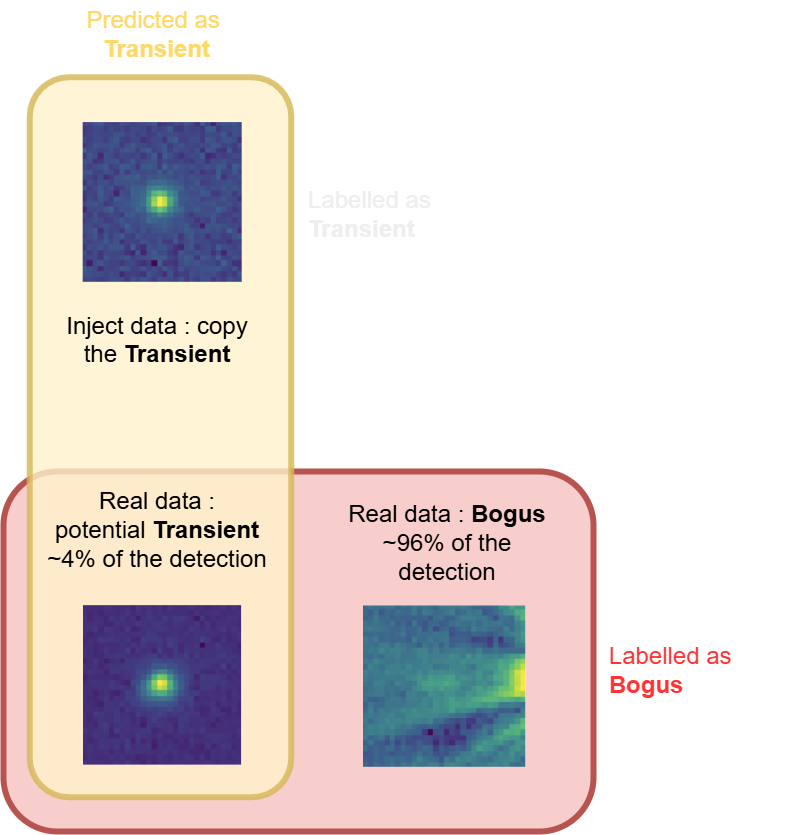
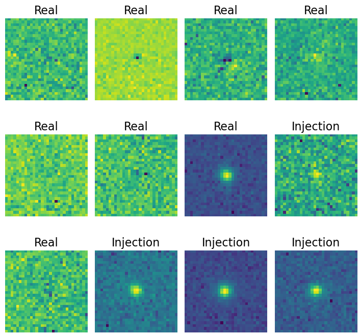
Training Data Presentation
The HSC RC2 subset is composed of 6 detectors, with 8 visits per filter.Producing the Cutouts:
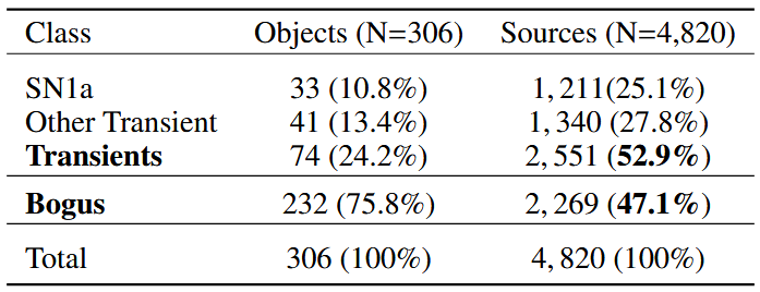
Classes and Labels:
Evaluation Data Presentation
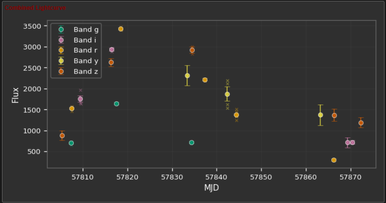
Filtering steps: from 8M to 342 LCs
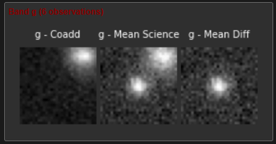
Human labeling:
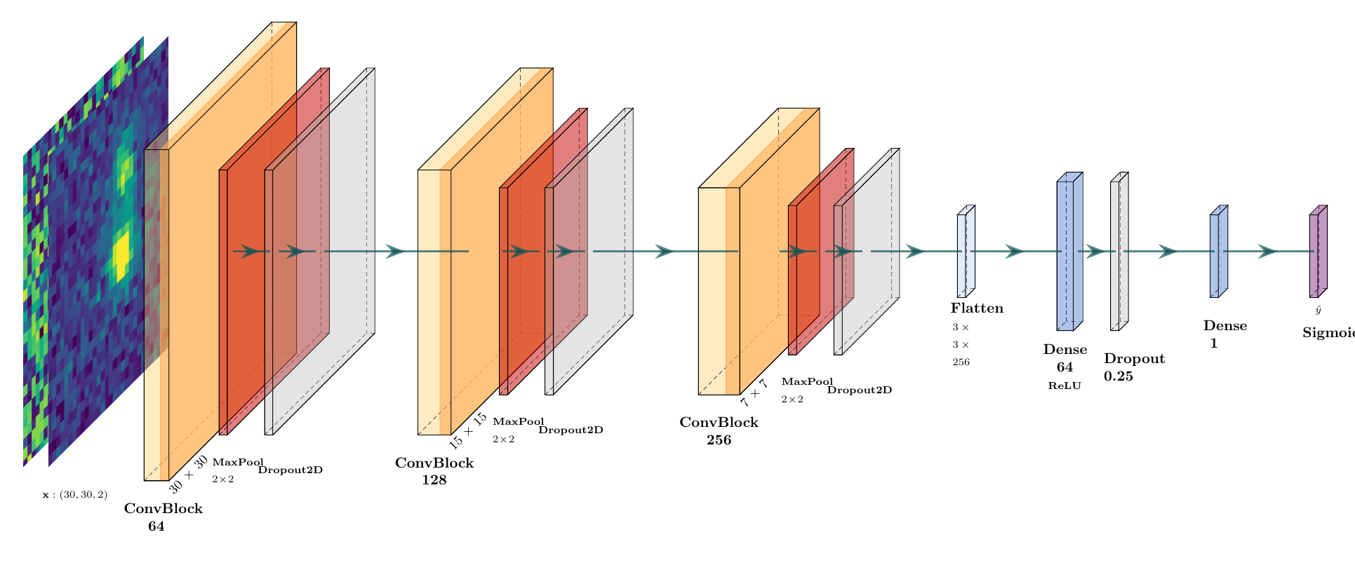
Network Architecture
Co-Teaching: A Self-Event-Selection Strategy for Weakly Supervised Learning
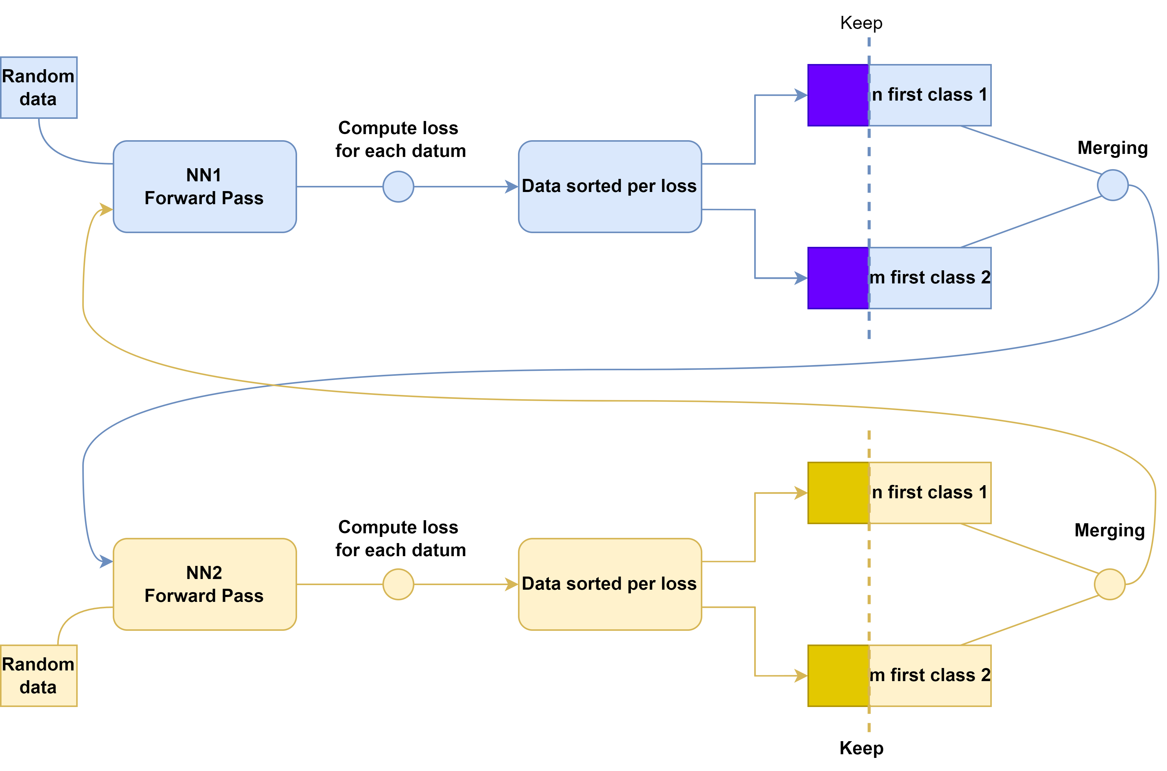
Two models are trained simultaneously with different views on the same dataset.


In each batch, each model selects the datum with the smallest loss (most confident predictions).
Avoid training on the wrong labels.
Pros:
- Effective for noisy datasets.
Cons:
- Increases computational cost.
- Assumes symmetrical noise.
Asymmetrical Co-Teaching
Two models are trained simultaneously with different views on the same dataset.

Key Changes:
- Implements different remembering rates for each class.
- Better fits the needs of our asymmetrically weakly supervised dataset.
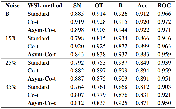
WSL analysis
DIA Calibration is expected to improve across time and survey conditions.
Four different training sets with varying noise levels.
Our method outperforms standard training, especially in the most noisy setting.
Ensembles and MC Dropout
Ensembles:
- Train multiple models with different initializations.
- Average predictions to reduce variance and improve robustness.
- Cost: T trainings and T inferences.

MC Dropout:
- Apply dropout during inference to simulate an ensemble of models.
- Perform multiple forward passes to estimate uncertainty.
- Cost: T inferences.

Predictive uncertainty (from variance of predictions):
\[ \hat{\mu}(x)=\frac{1}{T}\sum_{t=1}^{T}p_t(x), \qquad \widehat{\mathrm{Var}}(x)=\frac{1}{T-1}\sum_{t=1}^{T}\left(p_t(x)-\hat{\mu}(x)\right)^{2} \]
where \( p_t(x)=\begin{cases} \sigma(f_t(\mathbf{x}, \hat\theta_t)), & \text{for ensemble}\\ \sigma(f_t(\mathbf{x}, \hat\theta, z_t)), & \text{for MC Dropout} \end{cases} \)
UQ for Co-Teaching
Co-Teaching methods train two models simultaneously. Let's use them as an ensemble.
\( N=2\) ensemble is small, we can extend it by performing M stochastic forward passes with MC Dropout for each model, resulting in a total of \(N\times M\) predictions.
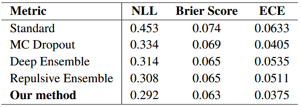
Metrics for Uncertainty Quantification
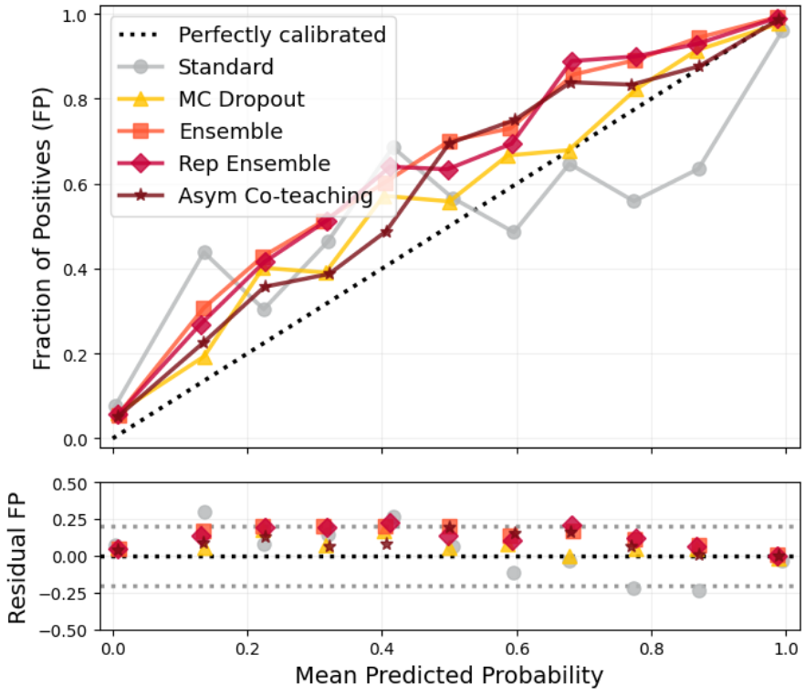
Calibration Metrics:
- Negative Log-Likelihood (NLL): quality of probabilistic predictions.
- Brier Score: MSE of probabilistic predictions.
- Expected Calibration Error (ECE): difference between predicted probabilities and observed frequencies.
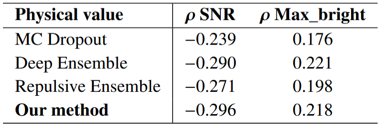
Correlations with Physical Quantities:
- Correlations with Signal-to-Noise Ratio (SNR).
- Correlations with maximum brightness of a SNIa.
\[ \rho = 1 - \frac{6 \sum d_i^2}{n(n^2 - 1)} \]
UQ analysis
Using UMAP for NN Latent Space visualization

UMAP Overview:
- Preserves both local and global structure using non-linear dimensionality reduction.
- Builds a nearest-neighbors graph and optimizes it for lower dimensions.
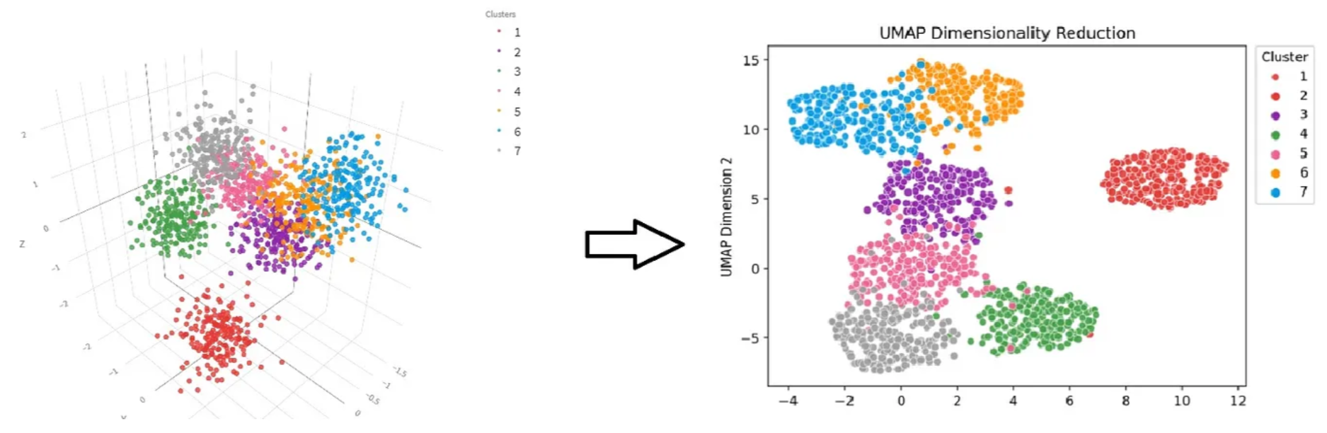
UMAP in our case:
Applied to the projection of inputs in the latent space of the network.UMAP Results
UMAP Results: SNR overlay
UMAP Results: UQ overlay
Outcomes of the project
- New Asym-Co-Teaching methods that allow mitigation of the risk in a high-stakes class.
- Novel uncertainty quantification method for Co-Teaching, providing better-calibrated uncertainties at lower cost.
- UMAP visualization of the latent space confirms our interpretation of global model behavior.
- Further exploration of the latent space to identify specific features or patterns associated with the bogus class.
- Expanding this work to upcoming datasets.
- Exploration of the systematic performance of MC–ensemble mixtures.
Shapley Values meet NNPDF
Raphaël Bonnet-Guerrini1, Stefano Carrazza2, Dakshansh Chawda 2, Stefano Forte2, Eva Groenendijk2, Vincenzo Piuri1, and Ramon Winterhalder21Computer Science Department, University of Milan; 2Physics Department, University of Milan

Parton Distribution Functions (PDFs) and NNPDF
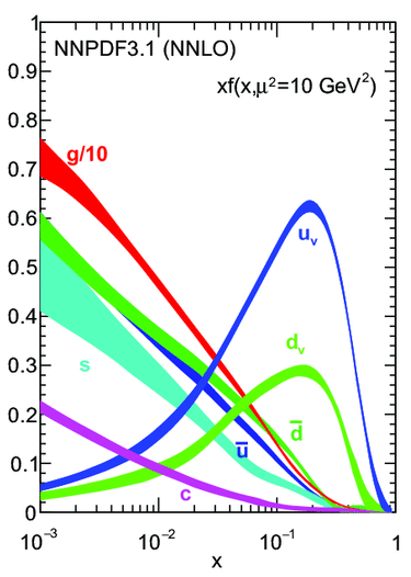
- Describe the probability of finding a parton carrying a fraction \(x\) of the proton's momentum at a given energy scale \(Q^2\).
- Essential for predicting outcomes of high-energy particle collisions.
- NNPDF uses neural networks to model PDFs without assuming a specific functional form.
- Trained on experimental data from different detectors.

NNPDF: an inverse problem
NNPDF solves an inverse problem: we have a set of experimental data and we want to find the underlying PDFs that best explain the data.
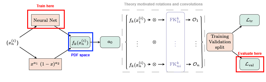
Theory (QCD, QED, EW) allows us to compute the observable values \(\mathcal{O}_n\) from the PDF space, and the inverse is done by fitting precise experimental data from the LHC.
PDF space
The PDF space is a high-dimensional space (flavor basis or evolution basis).
Why does a given flavor look like this in a given \(x\) region? Which datasets are responsible for this behavior?
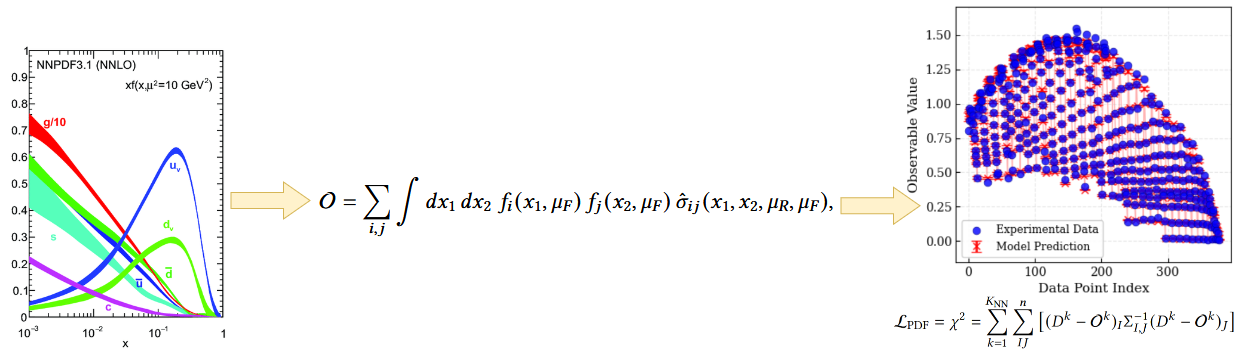
Makes it difficult to perform systematic tests and obtain a clear understanding of each flavor on the fit.
NNPDF a black box model ?
Black-box systems are a recurrent interpretability issue in modern DL. We can take inspiration from the methods developed there to solve the interpretability problem of NNPDF.
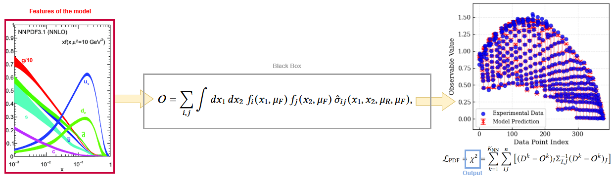
XAI answer : What's the impact of one feature on the output of the model ?
Shapley Values
Inherited from game theory: represent the value of the contribution \(\phi\) of a player \(i\) within a coalition \(S\).
\[ \phi_i = \sum_{S \subseteq N \setminus \{i\}} \frac{|S|! \, (|N| - |S| - 1)!}{|N|!} \left[ v(S \cup \{i\}) - v(S) \right] \]where \(N\) is the set of all players, \(S\) is a subset of players not including \(i\), and \(v(S)\) is the value of the coalition \(S\).
Computational cost as scales exponentially with the number of players \(2^N\).
SHAP adapt SV for DL application. Makes them computable for high amount of players (features) given certain assumptions and approximations.

Shapley Value, the perfect closure test metric?
Applying Shapley Values to NNPDF, we treat each flavor as a feature of our black-box model.
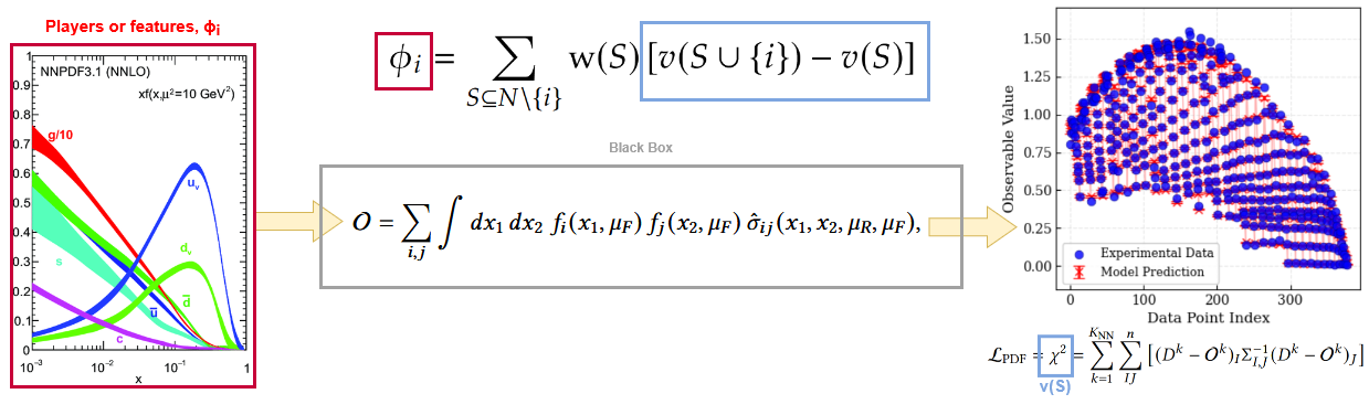
- \(\phi_i\) is the Shapley Value for flavor \(i\).
- \(N\) is the total number of flavors.
- \(S\) is a subset of flavors not including \(i\).
- \(v(S)=\chi^2\) is the value of the coalition when all flavors in coalition \(S\) are perturbed, while \(i\) and the rest of the flavors remain untouched.
How to perturb the PDF space ?
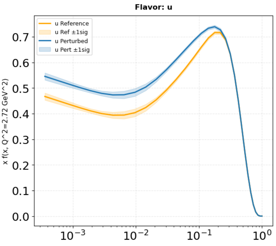
- Width and amplitude of the bump ?
- Location of the bump ?
- How to respect the physical constraints of the PDF ?
- Proportional perturbation across flavors ?
Coalitions and complexity
What we compute: the exact Shapley value for each PDF flavor by averaging its marginal contribution across all coalitions (all subsets of flavors).
Computational cost: exponential in the number of flavors, as we need to evaluate the fit for each coalition. In the flavor basis, \(N=9\) flavors, we have \(2^9 = 512\) coalitions.
Using exact Shapley values, we make no assumption of independence of the features.
How to interpret the SV?
\(x\) region dependency: Perturbation is local and we can expect different contributions for different \(x\) regions.
Dataset dependency: \(\chi^2\) which is computed based on experimental dataset. We expect different contributions for different datasets.
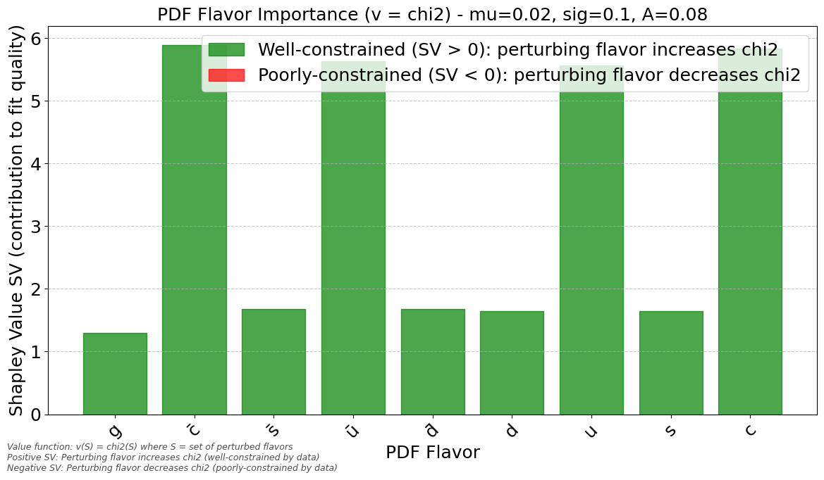 Exact Shapley Value have a completeness property:
\[\sum_{j \in N} \phi_j = v(N)-v(\emptyset)\]
and \(v(s)=\chi^2\) so they share the same unit.
Exact Shapley Value have a completeness property:
\[\sum_{j \in N} \phi_j = v(N)-v(\emptyset)\]
and \(v(s)=\chi^2\) so they share the same unit.
Next steps
- Implementation for proton-proton collisions (for now only implemented for DIS).
- Implementation in NNPDF.
- Perturbations respectful of physical constraints.
- Systematic study of the SVs' behavior for different perturbations and datasets.
Mechanistic Interpretability for a Neutrino Foundation Model
Raphaël Bonnet-Guerrini1, Johann Ioannou-Nikolaides2, Troels Petersen2, Vincenzo Piuri 1, Jean-Loup Tastet2 and Inar Timiryasov21Computer Science Department, University of Milan; 2Physics Department, Københavns Universitet, Denmark
Foundation models
Foundation models are large-scale machine learning models that are trained on a wide variety of data and can be adapted to a wide range of downstream tasks. They have shown remarkable performance in various domains, including natural language processing, computer vision, and more recently, in scientific domains such as physics.
Most foundation models rely on two specificities:
- The self-attention mechanism of the Transformer architecture.
- The available volume of data and the possibility to perform Self-Supervised Learning.



Foundation model in Neutrino Physics
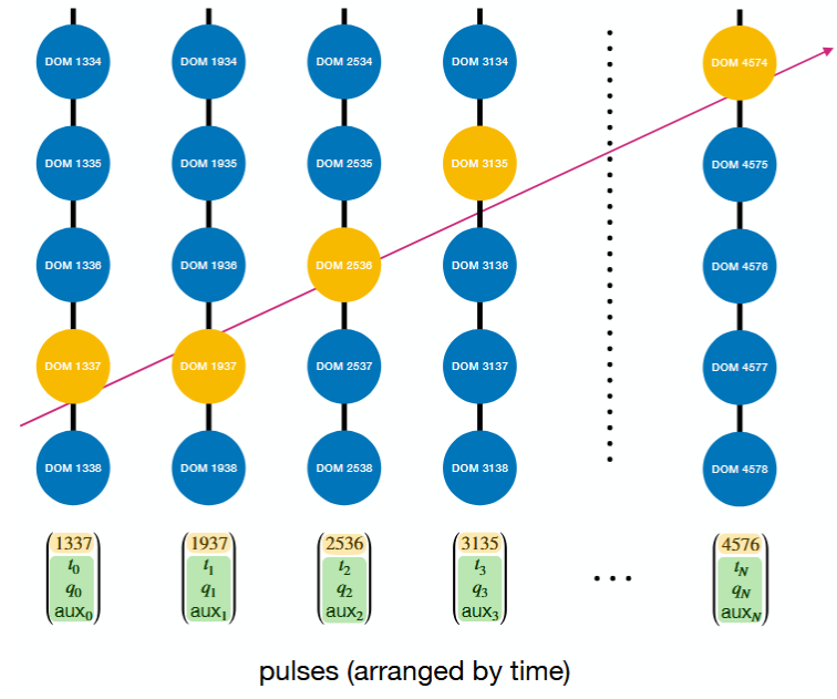
Neutrino detectors record pulses.
A pulse is a time series of the light emitted by the interaction of a neutrino with the detector.
It tracks the recorded time, the directions and the energies of the incoming neutrinos.
PolarBERT is a foundation model trained on 131,000,000 high-quality Monte Carlo neutrino events.
Downstream tasks include classification or reconstruction of the energy and direction.

Interpretability at the era of Foundation Models
Foundation Model are able to generalize.
Mechanistic Interpretability asks: ⇨ How did my model solve this general class of problems?
One of the methodological approaches is to reverse engineer the model, identifying what is the function of each part.
Natural decomposition (Neurons, Layers, Attention heads) fails because of polysemanticity caused by superposition (#feature>#neurons).

Sparse representations and Latent Spaces
Polysemanticity is caused by overlapping directions in the activation space. Dimensionality reduction techniques may not be able to disentangle the features.
To overcome this we can use Sparse Dictionary Learning (SDL) to find a sparse representation of the latent space.
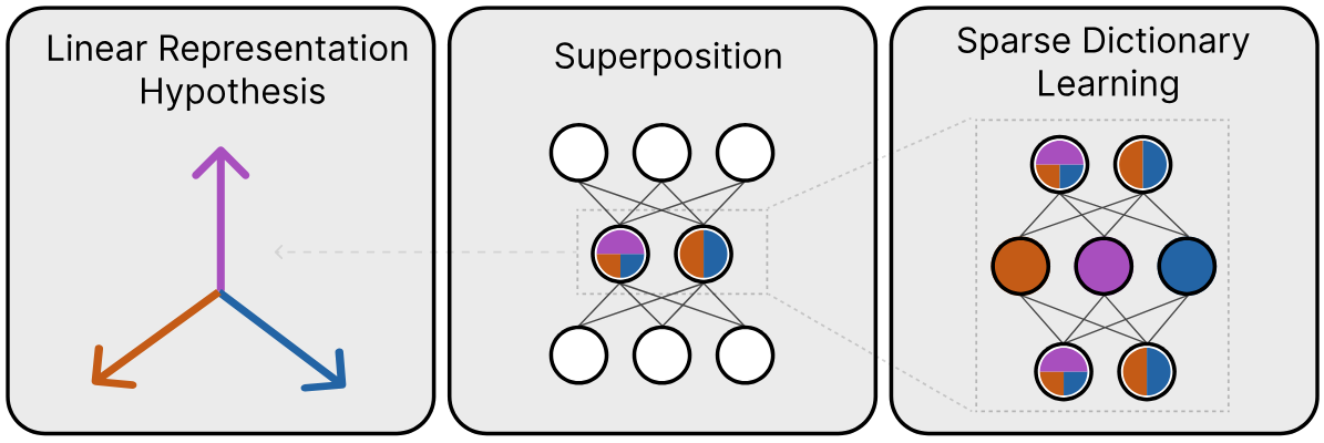
This allows the identification of behavior in the sparse latent space, providing insight on the network comprehension of underlying physics.

Potential behavior to investigate
- Are there specific regions for very long vs very short inputs?
- Muon vs neutrino tracks.
- Does the model learn to identify the different light patterns of different neutrino flavors?
Any of your ideas!
Backup Slides
Asymmetrical Co-Teaching
Calibration Metrics
- Negative Log-Likelihood (NLL): quality of probabilistic predictions.
- Brier Score: MSE of probabilistic predictions.
- Expected Calibration Error (ECE): difference between predicted probabilities and observed frequencies.
Shapley Values Pseudo code
# INPUT: observables, mu,sigma,amplitude, n_samples, n_flavors = n
# OUTPUT: shapley_vals[], baseline_chi2, cache

baseline_chi2 = evaluate_chi2(observables, flavor_subset=[])   # v({})

cache = {}   # map subset -> v(S)
all_subsets = power_set(0..n-1)     # exclude full-set if desired

for i in 0..n-1:
SV = 0
for S in all_subsets:
    if i in S: continue

    # v(S)
    if S not in cache:
    cache[S] = evaluate_chi2(observables, flavor_subset=list(S), mu,sigma,amplitude, n_samples)
    vS = cache[S]

    # v(S ∪ {i})
    S_with = S ∪ {i}
    if S_with not in cache:
    cache[S_with] = evaluate_chi2(observables, flavor_subset=list(S_with), mu,sigma,amplitude, n_samples)
    vSw = cache[S_with]

    Δ = vSw - vS                                   # marginal contribution
    s = |S|
    w = factorial(s) * factorial(n - s - 1) / factorial(n)
    SV += w * Δ

shapley_vals[i] = SV

# RETURN: shapley_vals, baseline_chi2, evaluated_coalitions=|cache|
# COMPLEXITY: time ~ O(n · 2^n · cost_eval), space ~ O(2^n) (memoized)
Shapley Values weight
In game theory, Shapley Values represent the contribution \(\phi_i\) of a player \(i\) within a coalition \(S\) by comparing the outcomes of scenarios where the player is present \(v(S \cup \{i\})\) versus absent \(v(S)\). \[ \phi_i = \sum_{S \subseteq N \setminus \{i\}} \text{w}(S) \left[ v(S \cup \{i\}) - v(S) \right] \label{eq:comb_SV} \] With: \[ w(S) = \frac{|S|! \, (|N| - |S| - 1)!}{|N|!} \] \(w(S)\) weights for the importance of the coalition \(S\) being tested. It is the probability that the set of players who come after \(i\) is exactly \(S\).- \(|S|!\) is the number of ways to order the predecessors of \(i\)
- \((|N| - |S| - 1)!\) is the number of way to order the players after \(i\)
- \(|N|!\) is the number of way to order all players
Shapley Values weight
This result is derived in the following way: Given \( |N| = n \), for a fixed player \(i\), let \( S \subseteq N \setminus \{i\} \) with \( |S| = s \). The probability that player before \(i\) are exactly \(S\) can be decomposed into two conditions: First, \(i\) can be in any position in \(N\), so: \[ p(\text{pos}_i = s+1) = \frac{1}{n} \] Second, given that \( i \) is in position \( s+1 \), the \( s \) players before \( i \) form a uniformly random subset of the remaining \( n-1 \) players of size \(\binom{n-1}{s}\): \[ p(\text{predecessors} = S \mid \text{pos}_i = s+1) = \frac{1}{\binom{n-1}{s}} \] To fulfill these conditions, we multiply those probabilities: \[ \frac{1}{n}\cdot \frac{1}{\binom{n-1}{s}} = \frac{1}{n}\cdot \frac{s!(n-1-s)!}{(n-1)!} = w(S) \]Thank you !